Dept. of Software Development, Monash University,
Melbourne, Australia
timm@cse.unsw.edu.au
- Simon Goss
Air Operations Division, Aeronautical & Maritime
Research Laboratory, Melbourne, Australia.
simon.goss@dsto.defence.gov.au
Tim Menzies
Dept. of Software Development, Monash University,
Melbourne, Australia
timm@cse.unsw.edu.au
-
Simon Goss
Air Operations Division, Aeronautical & Maritime
Research Laboratory, Melbourne, Australia.
simon.goss@dsto.defence.gov.au![]()
Tue Oct 1 16:38:50 EST 1996
This file is also available in postscript form.
Informal vague causal diagrams such as Figure 1 are a common technique for illustrating and sharing intuitions about a domain. Normally, such diagrams are viewed as precursors to other modeling techniques. That is, the standard approach is to continue the analysis process till the vagueness goes away.
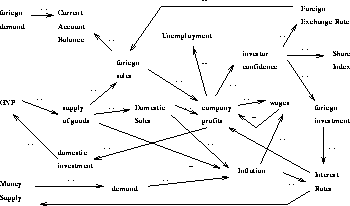
Figure 1: An economic vague causal diagram; from [5].
Here, we take another approach and explore what we can do with these vague diagrams without requiring precise analysis. Our approach is useful for both the acquisition and maintenance of knowledge. Standard software engineering methodologies are typically prescriptions on how to develop some initial system. Here we formalise the process of handling an existing, possibly poorly understood, system. Our goal is the structuring and the optimisation of the resources available during the maintenance phase. In the usual case, software maintenance is the process of understanding someone else's idiosyncratic code which may or may not be documented. An extreme software maintenance problem occurs when handling legacy systems where the maintainer may not even have access to the source code.
Vague models must be processed differently to standard software systems. The standard software design activity cycle shown in Figure 2 [11]. Logical design comprises a brainstorming elicitation stage followed by a representation stage that systematises the concepts found during elicitation. To make the representations exhibit behaviour, they must be transformed into a lower-level representation which can be operationalised. During this transformation stage, implementation-dependent details will contort the representation. Once operationalised, these concepts can be executed and tested. Testing can be divided into verification (i.e. was the system built right?) and validation (i.e. was the right system built?). Feedback from the testing process can improve the physical and logical designs.
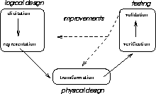
Figure 2: The design activity cycle;
adapted from [11]
In modeling of vague domains (see §2.1), systems development spends more time in testing and correction than initial logical design. Hence, development should move through the logical design stage as quickly as possible since most of the specification will be found in the testing stage. Vague modeling cannot produce correct models. Rather, it can only produce models that contain portions that are useful for known purposes.
Our preferred test engine is the HT4 abductive validation engine (summarised in §2.2). Previously, we have discussed HT4 and its applications to KBS inference and verification [18,17]. This article maps these low-level discussions into the high-level processes referred to in Figure 2. At its core, HT4 maps a theory down into a directed graph expressing the connections and invariants between entities in the theory. This low-level data structure, we will argue, is a unifying framework for operationalising most of the vague modeling process.
Figure 3 shows our proposed design activity cycle for vague domains. Elicitation (§3.1) lets us articulate and represent (§3.2) our theory; a library of desired behaviour (called the observations); and a success criteria for judging between competing inferences. In the transformation stage (§3.3), we:
 (§3.3.2).
 assessment operator
(§3.2.3).
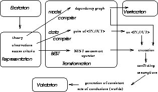
Figure 3: Vague Modeling: the Details
At execution time, each  pair is processed.
Portions of the dependency graph are extracted that connect members of
 back to members of
  . Recall that we are executing
vague models. Vague models are necessarily incomplete;
i.e. they are under-specified. When executing such under-specified
models, guesses have to be made and mutually exclusive guesses must be
managed separately. The extracted portions of the dependency graph
must be divided into internally consistent worlds.
The generation and assessment of the these worlds is a framework for
many expert system inference tasks, including validation. Good
theories can generate worlds that contain most of
  ; i.e. they
can explain a majority of the known behaviour.
Vague models contain inaccuracies. Therefore, vague modeling is only possible when the theory can be tested. That is, the computational properties of the validation engine constrain the modeling process; i.e. if we can't test it then we shouldn't model it. We will note below where the limits of the test device constrain the design process.
In order to explicate our argument, we begin with some background material about example vague domains (§2.1) and abduction (§2.2).
Elsewhere [15], we have characterised vague domains as: (i) poorly measured, i.e. known data from that domain is insufficient to confirm or deny that some inferred state is valid; (ii) hypothetical, i.e. the domain lacks an authoritative oracle (e.g. a person or a large library of known behaviour) that can declare knowledge to be ``right'' or ``wrong''; (iii) Indeterminate, i.e. inferencing over a knowledge base could generate numerous, mutually exclusive, outcomes.
The approached proposed here was developed by the first
author for a neuroendocrinological domain (§2.1.1) which we
would describe as the analysis of perturbations of an equilibrium
system![]() .
Our current goal is to test the generality of that previous
work approach in the domain of black-box comprehension (§2.1.2).
We would describe the air traffic control simulators found in this
second, black-box comprehension domain as spatio-temporal reasoning
over non-equilibrium systems. Note that our work in this second
black-box comprehension domain is still in its preliminary stages.
.
Our current goal is to test the generality of that previous
work approach in the domain of black-box comprehension (§2.1.2).
We would describe the air traffic control simulators found in this
second, black-box comprehension domain as spatio-temporal reasoning
over non-equilibrium systems. Note that our work in this second
black-box comprehension domain is still in its preliminary stages.
Neuroendocrinology is the study of the interaction of glands and nerves. Obtaining values for certain chemicals within the body is not as simple as, say, attaching a volt meter to an electric circuit:
 ).
).
Measurement in this domain can therefore be an expensive process and
not all entities are fully measured. For example, in
studies [17,8] of a sketch of a model of glucose
regulation [23], data was collected from six journal
articles. This sketch was represented as a compartmental
model ![]() . In all, none of the flow constants
were known and only 39% of the compartments were measured and not all
at the same time interval.
. In all, none of the flow constants
were known and only 39% of the compartments were measured and not all
at the same time interval.
Operations Research makes extensive use of large complex
simulation models. These can be the result of many person-years of
development and incorporate modules obtained from external sources. It
is common that such a system may be obtained from a third party.
Typically, some group called  derives some model
  representing their initial understanding of a problem (e.g.
modeling the performance of a missile system). This model is
operationalised in some third generation language to become
  .
Perhaps an attempt is made to document
  in a manual
 which may be incomplete.
 and
and  are then shipped to another
site where a second team (
 ) tries to understand them.
Conceptually,
  builds
  , a model representing the
local understanding of
  and the incomplete
  .
.
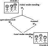
Figure 4: Commissioning Remote Models
The effort required to use  with confidence can be non-trivial,
especially when object code is supplied
without source code or access to the author.
Current
practice is for
  to be documented in an incomplete manner
(e.g. some procedural manual advising parametric sensitivity and
constants relating to the local physical and operational environment).
 can be regarded as a black-box model that
  must convert
(with some support from
  ) into a gray-box model
 . Once validated,
  would be used for planning, prediction, and
optimisation studies. However, first it is essential that we can
validate
the vague model
  since
local conditions may invalidate
 .
For example, the Australian Defence Forces use aircraft in
configurations that are different to how they are used overseas.
Certain parameters representing important domain knowledge
are stored in compiled numerical matrices and are
inaccessible to
  . For example,
these parameters may (i) be based on experimental
data from tests in other climates or (ii) contain
certain tacit assumptions about
aircraft operation.
Prior to relying on
 ,
,  would like to validate this model under local
conditions.
Elsewhere [18], we have given a precise overview of abduction.
Here, we offer an approximate characterisation of abduction as the
search for consistent subsets of some background theory that are
relevant for achieving some goal. If multiple subsets can be
extracted, then a preference operator (which we call  and
Bylander et. al. [2] call the plausibility operator pl)
must be applied to select the preferred subset(s). Abduction is
different to deduction. In deductive inference, all consequences of
known literals must be found by the inference procedure. In
abduction, the inference engine can ignore parts of the background
theory if they are not relevant for the current goal.
Abduction is a very general process. Abductive frameworks for various KBS tasks have been defined by numerous researchers; e.g. frame-based reasoning [20], Bayesian reasoning [2], diagnosis [6], explanation [13], and default reasoning [21]. We have also argued that abduction is also useful for planning, monitoring, verification, prediction, classification, qualitative reasoning [18], and validation [17]. The reason for this generality is that the processing of subset extraction is a synonym of known general frameworks for expert systems; i.e. Breuker's [1] components of solutions and Clancey's [4] situation-specific models [18]. For example, the formal difference between heuristic classification and heuristic construction [3] is the extraction of one subset or multiple conflicting subsets, respectively.
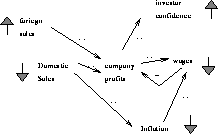
Figure: A portion of Figure 1.
In order to present a detailed example of abduction, we will run an example through our HT4 abductive inference engine [18]. A portion of Figure 1 is shown in Figure 5. The edge symbols of Figure 5 are explained in Figure 6.

Figure: Edge symbols of Figure 1 and
Figure 5.
In the case where  ={foriegnSalesUp, domesticSalesDown}
and
  = {investorConfidenceUp, inflationDown, wagesDown},
we can generate the following proofs
  for
for  :
:
 =
=
 ;
;
 =
=
 ;
;
 =
=  ;
;
 =
=  .
.
 . Continuing the example of
Figure 5, if
  =
=

 , then
{companyProfitsUp, companyProfitsDown} are assumptions. If we can't
believe that a variable can go up and down simultaneously,
then we can declare these assumptions
to be conflicting
(denoted
  ).
Hence
the key conflicting assumptions are the controversial
assumptions which are not dependent on other controversial
assumptions. In our example, these base controversial
assumptions
(denoted
  ) are all of our controversial assumptions.
We can used
  to find consistent belief sets called worlds
 . A proof
  is in
is in  if that proof does not
conflict with the environment
  (an environment is a
maximal consistent subset of
  ). In our example,
 ={companyProfitsUp},
 ={companyProfitsDown}. Hence,
 ={
={ ,
,  ,
,  } and
} and
 ={
={ ,
, 
 } (see
Figure 7)
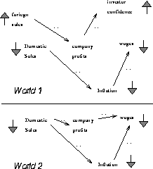
Figure: Worlds from Figure 5.
Which is the  world? We have argued elsewhere [18]
that, depending on the choice of
  operators, a variety of KBS
tasks can be emulated.
  operators can be defined for one of
three levels: vertex, proof, and world. When extending a proof from a
particular node, a vertex-level
  could elect to use
edges with the highest numerical rating. This could be used to emulate
a MYCIN-style certainty factor traversal. A proof-level
 could execute when some proofs or partial proofs are known;
e.g. beam search during planning. A worlds-level
  could execute when the worlds are known. Minimal-fault diagnosis is a
world-level
  assessment operator that returns world(s) which
maximise the number of
  puts obtained while minimising the
number of
  puts to those world.
  returns
the worlds(s) with the greatest overlap with known user profiles;
i.e. return the worlds a particular user is liable to understand. Our
preferred validation approach is a worlds-level
  that returns
the worlds that offer explanations for the most number of
 puts. This
  would therefore favour
 (which explains 3 members of
  ) over
  (which only explains 2 members of
  ).
).
The computational limits of the test engine constrains what can be
represented in vague modeling.
Elsewhere, we have explored the practicality of HT4 for medium
to large theories [17]. In our mutation study, 257
theories were artificially generated by adding random vertices and
edges to the and-or graph from a theory called Smythe '89![]() . These
were run using 5970 experimental comparisons. In the changing N
mutation study, the fanout was kept constant and the size of the model
was increased. Model size N was measured by the number of vertices
. These
were run using 5970 experimental comparisons. In the changing N
mutation study, the fanout was kept constant and the size of the model
was increased. Model size N was measured by the number of vertices
 in the ground graph. For example, foriegnSales
contributes three vertices to the ground graph: {foriegnSalesUp,
foriegnSalesSteady, foriegnSalesDown}. For that study, a ``give up''
time of 840 seconds was built into HT4. HT4 did not
terminate for
  in under that ``give up''time. We
conclude that the ``knee'' in the exponential runtime curve kicks-in
at around 800 literals. These result came from a Smalltalk V
implementation on a Macintosh Powerbook 170. A port to ``C'' on a
Sparc Station is underway.
The changing fanout mutation study examined the practicality of
HT4 for models of varying fanout (fanout is the number of edges
 that touch each vertex
  ; i.e.
 ).
In that study, the Smythe
'89 theory size was kept constant, but edges were added at random to
produce new graphs of larger fanouts. Six models were used of sizes
 .
At low fanouts, many
behaviours were inexplicable. However, after a fanout of 4.4, most
behaviours were explicable. Further, after a fanout of 6.8, nearly all
the behaviours were explicable [17].

Figure 8: Parameters from fielded expert systems.
From [19].
In practice, how restrictive is a limit of 850 vertices and
 ? The only reliable data we could
find on fielded expert systems is shown in
Figure 8 [19].
Figure 8 suggests that a practical inference
engine must work at least for the range
  and
and  . We therefore conclude
that vague modeling is practical for the size of expert systems seen
in current practice and for nearly the range of fanouts seen in
fielded expert systems. However, after a certain level of
inter-connectivity, a theory is able to reproduce any input/output
pairs. An inference procedure that condones any behaviour at all from
a theory is not a useful inference procedure. After the point where
%
  covered approaches 100%, vague modeling
becomes impractical.
Above, we have defined vague domains and the abductive framework that is the backbone of the process. We have explored the computational limits of validation in that framework. We can show where the testing process constrains the various stages of the design process; i.e. elicitation (§3.1), representation (§3.2), transformation (§3.3), verification (§3.4), and validation (§3.5).
The elicitation stage is an exploration of the domain. The goal of this stage is to make a first pass at discovering (i) list of terms for ``things'' in this domain; (ii) a rough idea of how these ``things'' influence each other; (iii) what ``things'' are incompatible (the invariants); (iv) a set of scenarios recording what behaviour your models should be able to reproduce.
In the elicitation, domain experts are encouraged to sketch out vague causal diagrams like Figure 1. Note that these models will be under-specified and can generate conflicts. At this stage, experts should not try and resolve these conflicts. Rather, their goal is to generate the set of all possible explanations that are acceptable to them. The process of extracting relevant and consistent subsets will be handled later.
Once drawn, the next stage in vague modeling is to walk through the
diagrams with scenarios; i.e. examples of how things impact the
system. These scenarios will later become our  puts and
our
  puts.
puts.
Tacit in the vague diagrams is invariant knowledge. For example, having said that inflation can go up or down is the statement that we can't believe that inflation can go up and down simultaneously. More generally, these diagrams can include invariants between any pairs of states. Invariants can be absolute or gradual:
 suntan=up.
 suntan.
When working with sensor data, it may be useful to introduce
summary nodes that generalise certain data. For example,
prolongedExposure to sunlight and sunLamps might both connect
to tanned; e.g.
prolongedExposure  tanned and
sunLamps
  tanned.
Vague causal diagrams can be generated from many pre-existing sources such as:
 B
to model proportionality and
A
  D to model
inverse proportionality.
Domains typically have pre-existing special constructs
which may be useful in elicitation of the vague causal diagrams.
For example,
neuroendocrinology using
compartmental models.
In compartmental models,
compartments are connected by ``pipes'' and each pipe has a flow
control
box. These flow rate through these flow controllers
can be changed by other compartments; e.g. glucose (a compartment)
can increase the glucagonProduction (a flow controller on a
pipe going into glucagon);
i.e.
glucose  glucagonProduction and
glucagonProduction
  glucagon.
Details of the test engine constrain the elicitation stage. In particular, we must restrict the size of vague models. In practice, this means avoiding low-level detail and removing time.
Avoiding low-level detail: Vague modeling is not a technique for recording of low-level detail since the HT4 inference engine has problems handling very big models (recall §2.2.2). Hence, if models get too big, we ne continuous variables with up, down, Steady; i.e. one of three states representing the sign of the change in those variables. Note that this introduces some indeterminacy into the model. Recall that in Figure 1, if foriegnSales and domesticSales go up and down respectively, then we have contradictory possible values for companyProfits ( up OR down). In vague modeling, we defer the resolution of these conflicts till the testing phase. In the meantime, recall that if HT4 generates multiple worlds for companyProfitsUp or companyProfitsDown, then these contradictory assumptions will be stored in multiple worlds.
Removing time:
 ,
,
 ,
,
 , .... Given T time ticks,
the practical limit to model size is the
limits noted in §2.2.2, divided by T. That is,
the longer the simulation, the smaller the model we can test.
In practice, for the current work, we plan to build our models without time. In the neuroendocrinological domain, time is removed by only using scenarios without time series data. This restriction still provides us with many data points. Much of the experimentation in neuroendocrinology is performed on separate groups of rats. Conclusions are made by comparing measurements in some control group to measurements in some treated group. In such scenarios, there is no sense of time flowing from the control group to the treated group.
In the black-box comprehension domain, time is harder to remove. Many of the systems in the target domain are large FORTRAN or C++ simulations which explicitly model time-series events. Our current approach in this domain is to develop an elicitation framework aimed at declarative representation. Time and position are often inter-changeable indexes in the navigation strategies of mariners and pilots. Traditional AI planning (e.g. STRIPS) avoids explicit representation of time by creating ordered lists representing priorities in schedules. We conjecture that pilot knowledge expressed in the this prioritised list framework, need not mention time. Rather, our rules will be reactions to some immediate situation rather than a reflection of some between-situations plan.
The representation stage fills in the details sketched in the elicitation stage. The goal of this stage is creation of (i) a theory (§3.2.1); (ii) some observations containing the scenarios that the theory should be able to reproduce (§3.2.2); and the success criteria (§3.2.3).
Smythe '87 [22] is a theory proposing connections between serum adrenocorticotropin ( acth), serum corticosterone ( cortico), and neuro-noradrenergic activity ( nna). Nna was measured as the ratio of noradrenaline to its post-cursor, 3,4-dihydroxphenyl-ethethyleneglycol. This theory is shown as the vague causal diagram of Figure 10. The temp vertex was introduced to model the user's statement that dex has the same effect as cortico.
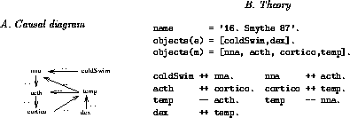
Figure 10: The Smythe '87 theory
The Smythe '87 theory is shown in Figure 10 in HT4 syntax. This theory starts with a name = 'a string' statement and is followed by two object statements. The object statements describe the events and the measures of the diagram. Events (denoted objects(e)) are like booleans while measures (denoted objects(m)) are for continuous variables. The body, which follows the head, contains the influence statements. The influence statements are pairs of measures connected by one of the topoi symbols (see Figure 6).
The Smythe '87 paper contains values comparing these values in various
experiments: (i) control i.e. no treatments; (ii) dex i.e.
an injection of dexamethasone at 100  ; (iii)
coldSwim i.e. a two minute swim in a bath of ice cold water; and
(iv) coldSwim, dex i.e. both a coldSwim and an injection
of dex. A sample of experimental results from Smythe '87 is
shown as the observations of Figure 11 (in HT4 syntax).
The experiments
are shown in the columns and the measures taken in the different
experiments are shown in the rows.

Figure: The observations for the Smythe '87 model
of Figure 10.
Our scenarios are comparisons between two experiments.
When we compare (e.g.) [coldSwim] to
[dex, coldSwim], we say that the input ( ) to scenario was
change(coldSwim)=arrived, change(dex)=arrived
and the output (
 ) of the scenario
was that acth=down,
cortico=down, nna=up.
The scenario
that our theory has to try and reproduce is
change(coldSwim)=arrived and change(dex)=arrived
leads to nna=up;
that is
cold swims and injections
of steroids increases stress levels in a rat.
The success criteria will be mapped into the HT4  operator. We use the success criteria to select preferred inferences.
Success criteria extract summaries of the inferences, and
then cull some inferences based on those summaries.
The exact
  operator is domain dependent. For
neuroendocrinology, we have used a
  operator that returns the
world(s) that cover the most
  puts. Note that this answers the
following question: ``can a theory of X reproduce known
behaviour of X?''. Elsewhere (§3.5) we describe
experiments were this was applied as a validation criteria which
successful found faults in published models of neuroendocrinology.
For other domains, (e.g. machine learning) we may chose to (i) return
the smaller worlds; (ii) the world(s) that make the fewest
assumptions; that (iii) use the least controversial assumptions; (iv)
the ``cheapest'' worlds (assuming that each edge is associated with
some notion of the cost of its inclusion); (v) etc.
The details of what can be represented are restricted by what can be handled at the transformation stage.
The physical design is the bridge between the logical design and an executable version which we can test. Specifically, the goals of the transformation stage is to be able to:
 put-
put- put
pairs. Each pair of <
 ,
, > is then passed
to the output of the data compiler (see §3.3.2)
for execution.
 assessment operator.
 operators have to be coded in the HT4
implementation language (Prolog).
Two styles of model-compilers are planned for the black-box comprehension domain. The first style is a generic partial-evaluator of rules with variables into the network of connections between literals in the rule. This partial-evaluator will need knowledge of the range of each field of each fact that can be asserted. The second style will be an attempt to ``shoe-horn'' the rule representation into the representation used in the neuroendocrinological domain. A hand inspection of the rules will be used to draw vague causal diagrams which will be mapped into the neuroendocrinological theory.
With the neuroendocrinological model compiler, if a vertex can be in one of N states, then one vertex is added for each such state. If an edge condones connections between two states of adjacent vertices, then an edge is added between those states. For example, power ++ lights is expanded into Figure 12.

Figure 12: Light is directly proportional to power.
All the vertices of Figure 12 are or vertices; i.e. belief in these vertices requires a belief in only one of its parents. The model compiler can add the disabling effects of rats via and vertices; i.e. vertices which we can only believe if we believe all their parents. For example, if we know that the rats in the basement disable the connection between the power and the lights (when they bump the cable), then we say if not rats then power ++ lights which expands into Figure 13.

Figure 13: The lights/power relationship works when rats are absent.
At this point, the neuroendocrinological model compiler gets intricate. A conjunction of competing upstream influences can combine to explain a steady vertex. Also, changes to an object's value downstream of an abler link can be explained in terms of changes to the abler. Returning to our rats, in the case of power not rising (but on) and the rats being present, the lights are dark. Now consider the same situation, but the rats suddenly disappearing. The lights going up can now be explained in terms of a change in the rat population. If we take these into account, we get Figure 14. In Figure 14 we include for the first time the incompatible vertices (see the double-headed arrows marked with a cross).
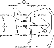
Figure 14: The final rats model.
For more details on the neuroendocrinology model compiler, see [16].
The data compiler converts tables like Figure 11 into  and
and  sets of vertices in the dependency graph. For example, in
the scenario [] to [dex] in Figure 11,
 = dex=arrived, coldSwim=absent and
  =
nna=up, cortico=down, acth=down.
There are five other scenarios:
< ,
, > pairs: [] to [coldSwim],
[] to [dex,coldSwim], [dex] to [coldSwim],
[dex] to [dex,coldSwim], and [coldSwim] to
[dex,coldSwim]. Therefore, we can
run six scenarios through the Smythe '87 model
of Figure 10.
Smythe '87 is a symmetrical model.
In symmetrical models, a comparison
from  to
to  is the same as
  to
to
 ; i.e. after studying [dex] to [coldSwim],
we do not need to study [coldSwim] to
[dex]. Non-symmetrical domains are those that include asymmetric
influences. Direct and inverse are symmetric influences
while ablers
are asymmetric. In asymmetric
domains, therefore, twice as many scenarios must be studied.
Verification is an exploration of the internal syntactic structure of a program. Preece, Shinghal and Batarekh [19] (hereafter, PSB) define a taxonomy of structural ``anomalies'' in rule-based expert systems (see Figure 15) and argue that a variety of verification tools target different subsets of these anomalies (perhaps using different terminology).
Some of these anomalies require meta-knowledge about knowledge base literals:
A rule is PSB-redundant if the same final hypotheses are reachable if that rule was removed. An unusable redundant rule has some impossible premise. A knowledge base is PSB-deficient if a consistent subset of askables leads to zero final hypotheses. A PSB-duplicate redundant rule has a premise that is a subset of another rule premise. PSB define duplicate rules for the propositional case and subsumed redundant rules for first- order case (where instantiations have to be made to rule premise variables prior to testing for subsets). PSB define ambivalence as the case where, given a consistent subset of askables, a rule-base cannot infer some final hypotheses.
PSB stress that the entries in their taxonomy of KBS anomalies may not be true errors. For example, the dependency network from a rule-base may show a circularity anomaly between literals. However, this may not be a true error. Such circularities occur in (e.g.) user input routines that only terminate after the user has supplied valid input. For this reason, the "errors" detected by internal testing are called anomalies, not faults. Internal test anomalies are used as pointers into the system which direct the developer to areas that require a second glance.
In vague domains, the anomalies shown in italics of Figure 15 are to be expected. For example:
However, a graph-theoretic analysis of the dependency
graph  can detect many of the other PSB anomalies:
 .
Find the roots and leaves of each component.
Compute the set intersection and set difference of the
askables with the roots and the final hypotheses with
the leaves.
An inspection of these sets will detect specification anomalies
Other useful verification studies are:
 , and those edges are already in
  , then that statement
is a duplicate of a previous statement.
Validation is an assessment of the program based on external semantic criteria. For each model generated from the logical design, we find:
 assessment operator that favours
world(s) that covers the most outputs (recall §3.2.3).
 was used when
processing the behaviour.
Edges that are never/rarely use can be reviewed with the
business users and (possibly) culled from the model.
In the case of competing models, we reject the models that explain
significantly less behaviour than their competitors. Returning to the
Smythe '87 theory (Figure 10), in the scenario
[coldSwim] to [dex, coldSwim], we can infer from
Figure 11 that  ={acthDown,corticoDown, nnaUp}
and
  = { change(dex)=arrived, coldSwim=present}. In
this comparison nnaUp can't be explained since their exists no
proof from nnaUp to
  which does not violate the proof
invariants. Another error can be found in the comparison [dex]
to [dex,coldSwim]. In this comparison
  =
{change(coldSwim)=arrived, dex=present} and
  =
{acthSteady, corticoUp, nnaUp} and only nnaUp can be
explained. What is interesting here is that the Smythe '87 theory had
been published in an international refereed journal [22]
and its validation errors were found by a detailed examination of the
data published to support it! Further, when these errors were shown to
the author of the theory, he found them novel and exciting; i.e. they
were significant errors.
Smythe '87 is a small theory. The Smythe '89 study explores how well abductive validation scales up to medium-sized models. Smythe '89 [23] is a theory of human glucose regulation. It contains 27 possible inputs and 53 measurable entities which partially evaluated into an and-or graph with 554 vertices and 1257 edges. Smythe '89 is a review paper that summaries a range of papers from the field of neuroendocrinology. Those papers offer 870 experimental comparisons with between 1 to 4 inputs and 1 to 10 outputs.
Smythe '89 was originally studied by QMOD, the technical precursor to HT4. That study found that 32% of the observations were inexplicable. QMOD could not explain studies or handle multiple causes. These restrictions implied that it could only handle of 24 possible comparisons. Even with these restrictions, QMOD found several errors in Smythe '89 that were novel and exciting to Smythe himself [8]. Like the Smythe '87 study, these errors had not been detected previously by international peer review.
When HT4 ran over the full 870 comparisons, it found more errors than
QMOD. Only 150 of the comparisons could explain 100% of their
 puts. On average, 45% of the
  s in those comparisons were
inexplicable. The level of critique offered by QMOD and HT4 is
surprisingly high. This is both a disturbing and exciting finding.
It is disturbing in the sense that if the very first large-scale
medical theory analysed by abductive validation contains significant
numbers of errors, then it raises doubts as to the accuracy of theories in
general. This result is exciting in the sense that the level of
critique is so high. Abductive validation promises to be a powerful
technique for theory review.
Vague modeling makes little use of two of the dominant themes in KA:
ontological engineering [10] and reusable problem solving
strategies (e.g. KADS [24]). While an
appropriate ontology may be useful for ``kick-starting'' the
elicitation stage, they may not be productivity tools for the rest of
the design activity life cycle in vague domains. Further, it is not
clear what (e.g.) KADS offers for the testing phase of a KBS. Our
framework easily supports validation and verification. While KADS has
a ``verification'' inference model![]() , in its current form it cannot be applied
reflectively on the KADS models themselves. Also, this KADS
``verification model'' makes no mention to assumption space
management; a technical issue that is central to our architecture and
validation process.
, in its current form it cannot be applied
reflectively on the KADS models themselves. Also, this KADS
``verification model'' makes no mention to assumption space
management; a technical issue that is central to our architecture and
validation process.
Vague modeling is the process of making what sense we can of half-formed ideas in a poorly measured domain. In this paper we have explored the design activity cycle of vague modeling based around vague causal diagrams and abductive inference. We have contrasted vague modeling with conventional modeling. In conventional modeling, most of the design is generated in the analysis stage. In vague modeling, most of the model is found during testing. Further, the limits of the computational device used in the testing phase restricts the modeling process back at the logical design phase. Hence, the test engine should be built first since, in vague domains, what can't be tested shouldn't be modeled. HT4 imposes two restrictions: the need to avoid low-level detail and the need for declarative representations that avoid time. Models that satisfy these restrictions can be verified and validated.
Originally, the approach described here was developed as a general approach, using the neuroendocrinology domain as an example. Our current task is to test the generality of this approach in the black-box comprehension domain. While the work done to date is preliminary, it has served to highlighted certain restrictions with the software developed for the neuroendocrinology domain. For example, we need better tools for building of model and data compilers (see §3.3.1 and §3.3.2). While ultimately these must be customised to a particular domain, model compilers for rules and frames should be added to the current system.
Some of the Menzies papers can be found at
http:// www.sd.monash.edu.au/  timm/pub/
docs/papersonly.html.
Vague Models and Their Implications for the KBS Design Cycle
This document was generated using the LaTeX2HTML translator Version 95.1 (Fri Jan 20 1995) Copyright © 1993, 1994, Nikos Drakos, Computer Based Learning Unit, University of Leeds.
The command line arguments were:
latex2html -split 0 words.tex.
The translation was initiated by Timothy Menzies on Tue Oct 1 16:37:53 EST 1996